
The Evolution of Frax Finance: The Pursuit of a Perfect Decentralized Stablecoin
TechFlow Selected TechFlow Selected
The Evolution of Frax Finance: The Pursuit of a Perfect Decentralized Stablecoin
This article will start with Frax's upcoming new version v3, systematically analyzing and reviewing each of Frax's full-stack products, guiding you to uncover the complete picture of Frax Finance.
🏆 The Holy Grail
Decentralized stablecoins face an impossible trilemma among capital efficiency, decentralization level, and price stability. Continuously seeking a balance among these three has become an aspirational yet difficult-to-achieve goal.
USDT and USDC excel in capital efficiency and price stability, enabling them to achieve massive market caps and widespread use cases, but they are highly centralized.
DAI, the longest-standing decentralized stablecoin, initially excelled in decentralization by relying primarily on ETH as overcollateralized assets. While this ensured price stability, it sacrificed capital efficiency, limiting its adoption and market scale compared to centralized stablecoins. Later, DAI gradually accepted centralized assets as collateral, trading decentralization for increased market cap.
UST is the most controversial decentralized stablecoin—achieving extreme capital efficiency while maintaining decentralization traits, briefly reaching a market cap second only to USDT and USDC. However, its aggressive strategy led the stablecoin into a death spiral under extreme conditions.
To date, no "perfect" decentralized stablecoin exists—this may be the "holy grail" that builders relentlessly pursue.

Frax Finance is a full-stack protocol centered around a decentralized stablecoin. Starting as a partially collateralized algorithmic stablecoin, it has gradually transitioned toward full collateralization while maximizing capital efficiency improvements. It has expanded horizontally into multiple domains, ultimately forming a matrix-like, full-stack DeFi ecosystem driven by its stablecoin. It is also the longest surviving non-fully-collateralized stablecoin.
Its product suite includes:
-
FRAX stablecoin: Decentralized USD stablecoin ★
-
FPI: Inflation-resistant stablecoin pegged to a basket of commodities ★
-
frxETH: LSD ★
-
Fraxlend: Lending ★
-
Fraxswap: Time-weighted decentralized exchange ★
-
Fraxferry: Cross-chain transfer ★
-
FXS & veFXS: Governance module ☆
-
AMO: Algorithmic Market Operations controller ★
-
Frax Bond - Bonds (v3 launching soon) ☆
-
RWA - Real World Assets (v3 launching soon) ☆
-
Frax Chain - Layer2 (not launched) ☆
Since launch, Frax has evolved through three versions—v1, v2, and v3. Unlike many protocols, each version of Frax involves not just functional upgrades but also major strategic shifts. Missing any version could mean fundamentally misunderstanding Frax.
-
Frax v1: Aimed to become an algorithmic stablecoin using "fractional algorithms" to gradually reduce collateral ratio and maximize capital efficiency.
-
Frax v2: Strategically abandoned the path of reducing collateral ratios, instead increasing collateralization toward full backing. Developed AMO to join the Curve Wars for on-chain liquidity governance, and launched frxETH into the Ethereum liquid staking derivatives (LSD) space.
-
Frax v3: Introducing real-world assets (RWA), continuing to leverage AMO across on-chain and off-chain liquidity.
This article begins with Frax's upcoming v3 release, analyzing and organizing Frax’s full-stack products to reveal the complete picture of Frax Finance.
Frax Finance v3
Frax v3 is an upcoming version whose core will revolve around RWA, while continuing to use AMO from v2 to gradually make FRAX a fully exogenous-collateralized, multi-asset decentralized stablecoin capturing both on-chain and off-chain value.
Fully Exogenous Collateralization
According to the FRAX balance sheet, the current collateral ratio (CR) of FRAX is 91.85%.
CR = (Owned assets + Lent assets) / Liabilities
CR = (615,357,001 + 65,654,459) / 741,400,658 = 91.85%
Starting with Frax v3, the protocol will introduce real-world assets (RWA) to increase CR until CR ≥ 100%, ultimately achieving 100% exogenous collateral backing for FRAX. In fact, as early as February 2023, community proposal FIP188 halted the algorithmic stablecoin mechanism of FRAX and began using AMO and protocol revenue to gradually increase the collateral ratio CR:
FIP188
This proposal was landmark for Frax. From FIP188 onward, Frax permanently discontinued the "fractional algorithm" and "de-collateralization" functions, transitioning from a partially collateralized algorithmic stablecoin to a fully collateralized one. Key points of the proposal include:
-
The original Frax design included a "fractional algorithm"—a variable collateral ratio adjusted based on FRAX demand, allowing the market to determine how much external collateral and FXS were needed per FRAX to equal $1.00.
-
The fractional algorithm was stopped because the cost of being slightly under-collateralized far outweighed its benefits. Market concerns about even 1% under-collateralization exceed the need for 10% additional yield.
-
Over time, growth, asset appreciation, and protocol income will raise CR to 100%. Importantly, this proposal does not rely on minting additional FXS to achieve 100% CR.
-
Protocol revenue will be retained to fund CR increases, pausing FXS buybacks.
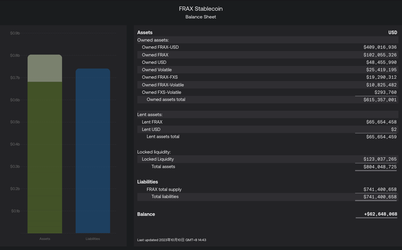
FRAX Balance Sheet 2023.10.10
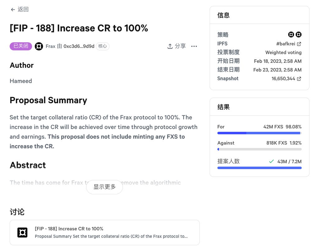
FIP 188 passed
RWA
As a key method to achieve CR ≥ 100% in Frax v3, the upcoming frxGov governance module will approve real-world entities, enabling AMO-controlled assets to purchase and hold real-world assets such as U.S. Treasuries.
Users can deposit FRAX into designated smart contracts to receive sFRAX—a mechanism similar to DAI and sDAI. Here's a comparison between sFRAX and sDAI:
-
sDAI yields slightly above average Treasury returns (currently 5%, up to 8%) because not all DAI holders deposit into the DSR contract. Maker’s RWA returns are distributed only to those who deposit DAI to earn sDAI, meaning a subset captures all RWA gains.
-
sFRAX shares this feature, but due to Frax accumulating large amounts of Curve and Convex tokens during v2 and securing voting power via lockups, it can allocate certain CRV and CVX rewards earned on-chain, boosting sFRAX's overall yield. Additionally, it can quickly shift between on-chain and off-chain allocations when returns or risks become unfavorable on either side.
IORB Oracle
FRAX v3 smart contracts adopt the Interest on Reserve Balances (IORB) rate set by the Federal Reserve to inform certain protocol functions, such as sFRAX yield accrual.
-
When IORB rates rise, Frax’s AMO strategy will heavily collateralize FRAX with Treasury bills, reverse repo agreements, and dollars deposited at Federal Reserve banks earning IORB.
-
When IORB rates fall, the AMO strategy will rebalance FRAX collateral using decentralized on-chain assets and collateralized loans from Fraxlend.
In short, FRAX v3 adjusts its investment strategy based on the Federal Reserve’s IORB rate—allocating funds to off-chain instruments like Treasuries when off-chain yields are high, and shifting to on-chain lending (e.g., Fraxlend) when on-chain yields are higher—to ensure maximum returns and stablecoin stability.
frxGov Governance Module
Frax v3 will remove multisig entirely, implementing governance solely through the smart contract-based frxGov module (veFXS). This marks a significant step toward decentralized governance.
FraxBond (FXB) Bonds
Both sFRAX and FXB bring Treasury yields into Frax, but differ:
sFRAX represents the zero-maturity segment of the yield curve, while FXB represents forward segments. Together, they form a comprehensive on-chain stablecoin yield curve.
-
If 50M FRAX is staked as sFRAX, approximately 50M USDC (assuming CR=100%) from reserves can be used off-chain to purchase short-term Treasuries worth $50M.
-
If 100M 1-year FXB bonds are sold for 95M USDC, the off-chain partner entity can use $95M to buy 1-year Treasuries.
Additionally, FXB is a transferable ERC-20 token that can build liquidity in secondary markets and circulate freely, offering users diverse stablecoin investment options with varying maturities, yields, and risk levels—and providing new composability components for DeFi legos.
Frax Finance v1
Frax v1 introduced the concept of a fractional-algorithmic stablecoin—partially backed by exogenous collateral (USDC) and partially unbacked (supported algorithmically by endogenous FXS).
For example, at a CR of 85%, each redeemed FRAX provides the user with $0.85 USDC and $0.15 worth of FXS.
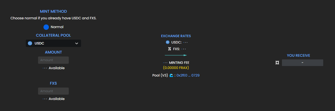
Minting $FRAX using USDC and FXS in Frax v1
In v1, AMO existed in its simplest form, known then as the fractional algorithm. Its main function was adjusting the CR during FRAX minting based on market conditions, originally scheduled at fixed intervals (e.g., hourly).
At launch, FRAX was minted at CR=100%—i.e., 1 FRAX = 1 USDC—called the "integer phase." Afterward, at regular intervals, the AMO would adjust CR up or down based on market data, entering the "fractional phase."
-
If FRAX > $1 and expansion is needed, CR decreases, allowing more FRAX to be minted with less collateral.
-
If FRAX < $1 and price falls below peg, CR increases, adding more backing per FRAX to restore confidence.
While the fractional algorithm influenced CR during new minting, its impact on the overall system CR was slow. To accelerate dynamic CR adjustments and align with desired levels, Frax v1 added two mechanisms:
Decollateralization and Recollateralization
-
Recollateralization: When the system raises CR, more USDC must be added. Frax incentivizes users: anyone can add $1 worth of USDC and receive $1.2 worth of FXS.
-
Decollateralization (Buyback): When CR decreases, users can exchange FXS for equivalent-value USDC directly from the system, after which FXS is burned. No bonus is offered in this mechanism.
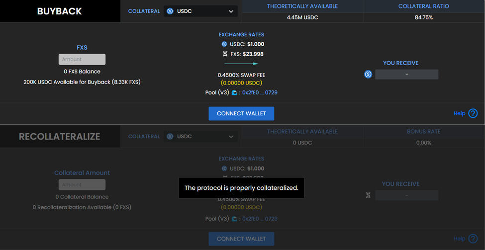
Decollateralization (Buyback) and Recollateralization interface

Frax v1 launched during the peak of algorithmic stablecoins in DeFi, alongside projects like Basis Cash and Empty Set Dollar (ESD). At the time, Frax was considered the most conservative among them. As market hype faded, Frax was the only survivor, later pivoting in v2 to increase collateralization and optimize treasury usage.
Frax Finance v2
Frax v2 was the most active version—discontinuing the fractional algorithm, launching AMO for treasury management, gradually filling the CR with profits, introducing new products like Fraxlend and frxETH, and emerging as a winner in the Curve Wars for on-chain liquidity governance.
AMO (Algorithmic Market Operations Controller)
AMO functions like the Federal Reserve’s monetary policy tool. As long as it doesn’t lower the collateral ratio or break the FRAX peg, it can execute arbitrary monetary policies—minting, burning, and allocating funds within predefined algorithmic limits. Thus, AMO performs algorithmic open market operations (hence its name), but cannot simply mint FRAX out of thin air to disrupt the peg.
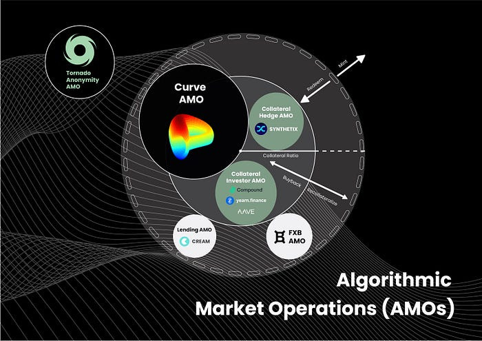
Currently, Frax operates four AMOs, with Curve AMO holding the largest capital. Through AMO, the protocol deploys idle treasury assets (mainly USDC), combined with algorithmically controlled FRAX minting, into other DeFi protocols:
-
Maximize treasury utilization to earn extra yield. For example, if the treasury holds 1M USDC, AMO mints 1M FRAX to create a USDC-FRAX LP pair, effectively earning yield on 2M in capital.
-
Since the minted FRAX belongs to the protocol and can be withdrawn and burned within AMO strategies before circulating to users, it has minimal impact on FRAX’s peg.
-
Increases FRAX’s market cap without adding new collateral.
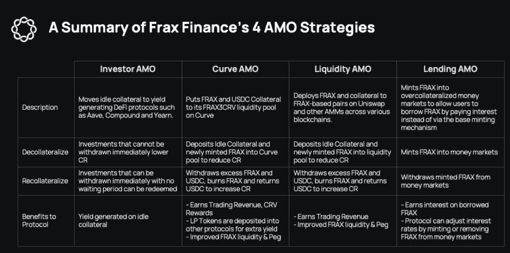
Take the Curve AMO strategy as an example:
-
Decollateralize: Deposit idle collateral and newly minted FRAX into Curve pools.
-
Recollateralize: Withdraw FRAX-USDC LP from pool, burn excess (protocol-controlled) FRAX, return USDC to boost CR.
-
Protocol Revenue: Accumulate trading fees and CRV rewards, periodically rebalance pools. Deposit LP tokens into platforms like Yearn, Stake DAO, and Convex Finance for additional yield.
Analyzing AMO’s crucial “money printing” capability
The core of AMO’s “money printing” strategy can be summarized as follows:
When AMO adds treasury USDC to a Curve pool, depositing a large amount alone would skew the pool’s ratio and affect price. Instead, pairing USDC with proportionally “printed” FRAX allows low-slippage entry, with LP tokens held and controlled by AMO.
Beyond this, another scenario enables maximal “printing”:
Let Y be the pre-“printed” FRAX supply, and X% be the market’s tolerance for FRAX dropping below $1.
If selling all Y into a Curve pool with Z TVL and amplification factor A causes less than X% price impact, then circulating Y amount of algorithmic FRAX is acceptable.
In other words, since Curve AMO controls LP in its own Curve pool, if FRAX drops X%, AMO can perform recollateralization—withdraw and burn excess FRAX—to boost CR and restore peg. The greater the LP controlled by AMO, the stronger this ability.
Therefore, before FRAX drops X%, we can calculate a safe amount of FRAX that can be sold into the Curve pool without significantly affecting price or triggering CR adjustments. This defines the maximum “printing” capacity.
For instance, a $330M FRAX3Pool can absorb at least a $39.2M FRAX sell order with less than 1 cent price movement. If X = 1%, then at least 39.2M algorithmic FRAX can circulate safely without breaking the peg.
This strategy creates a mathematically sound lower bound for circulating algorithmic FRAX—enabling powerful market operations without risking peg stability.
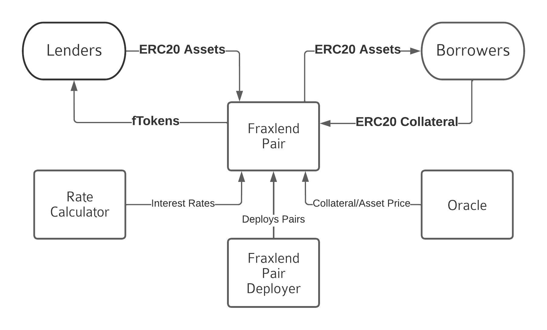
Fraxlend
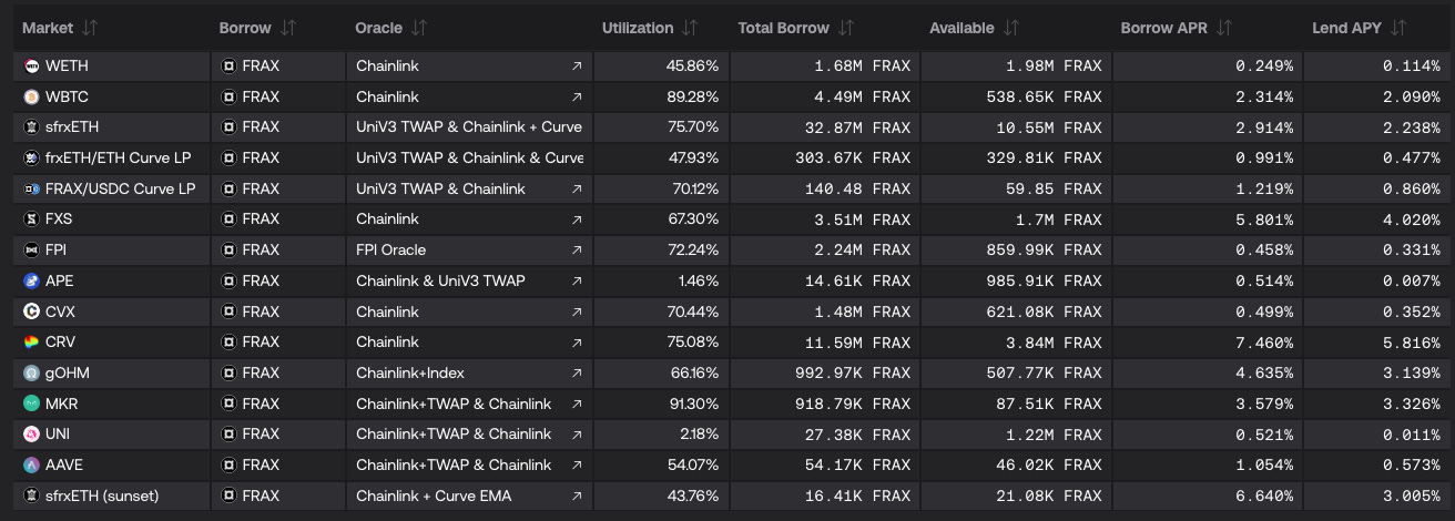
Fraxlend is a lending platform offering borrowing markets between ERC-20 assets. Unlike Aave v2’s pooled model, each lending pair in Fraxlend operates as an isolated market. When you deposit collateral for borrowers, you explicitly accept its value and risk. This isolation design has two key features:
-
Any issues related to collateral or bad loans are contained within individual pairs, not affecting other lending pools;
-
Collateral cannot be borrowed.
Fraxlend Mechanism – Interest Rate Model
Fraxlend offers three interest rate models (in practice, models 2 and 3). Unlike most lending protocols, all Fraxlend rate calculators auto-adjust based on market dynamics without requiring governance intervention. The Frax team believes market-driven rates are superior to slow governance proposals during volatility.
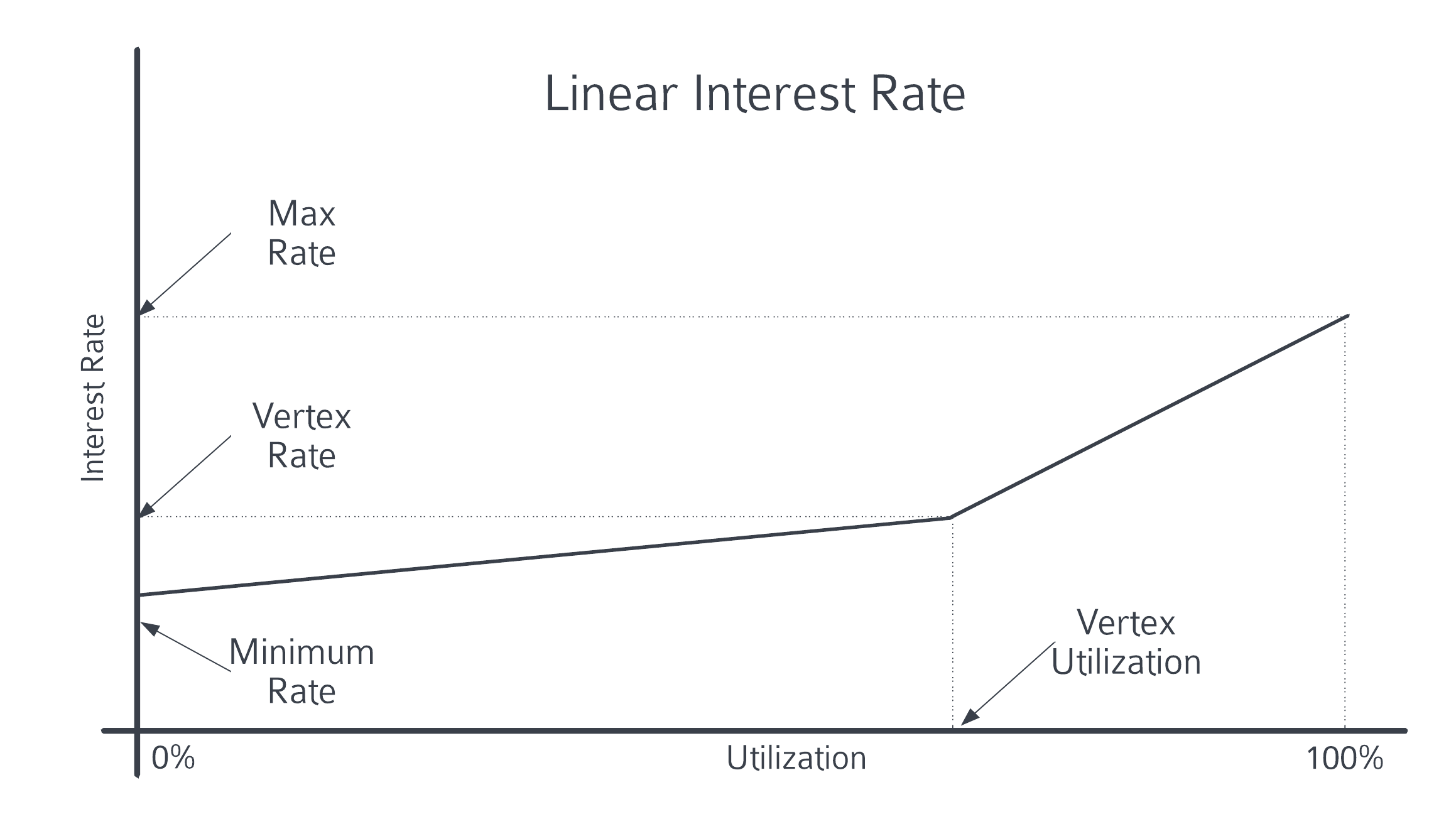
1 Linear Rate
When utilization exceeds a threshold, the rate curve steepens. Most lending protocols use this basic model—raising rates when pools are overused to incentivize deposits and repayments.
2 Time-Weighted Floating Rate
This model adjusts rates over time using three parameters:
-
Utilization: Adjusts rate based on fund usage.
-
Half-life: Determines adjustment speed. When utilization is high, rates multiply; when low, they decay.
-
Target Utilization Range: No adjustment occurs within this range—considered market-equilibrium.
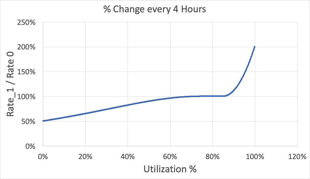
Currently, the rate half-life is 12 hours. At 0% utilization, the rate halves every 12 hours; at 100%, it doubles every 12 hours.
This rate model played a critical role in Curve founder Mich’s CRV liquidation event. Due to a 0-day compiler vulnerability in Vyper, Curve was exploited, leading to a run on Mich’s CRV loan position and lender withdrawals—pushing utilization near 80–100%. Fraxlend’s CRV market uses the time-weighted floating rate model: as utilization approached 100%, the 12-hour half-life caused borrowing rates to double every 12 hours, forcing Mich to repay promptly—or face imminent liquidation.
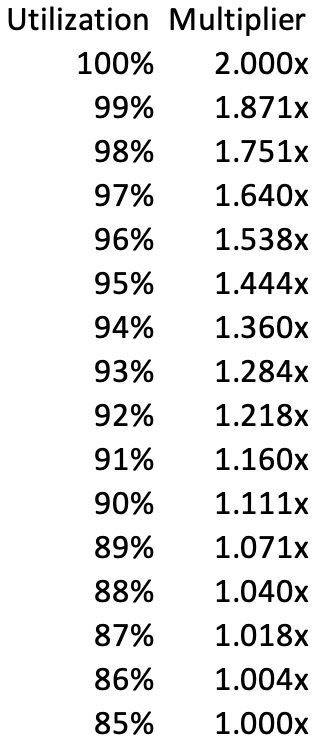
Rate adjustment multipliers at 85%-100% utilization
The chart below shows rate changes with a 4-hour half-life and target utilization range of 75%–85%:
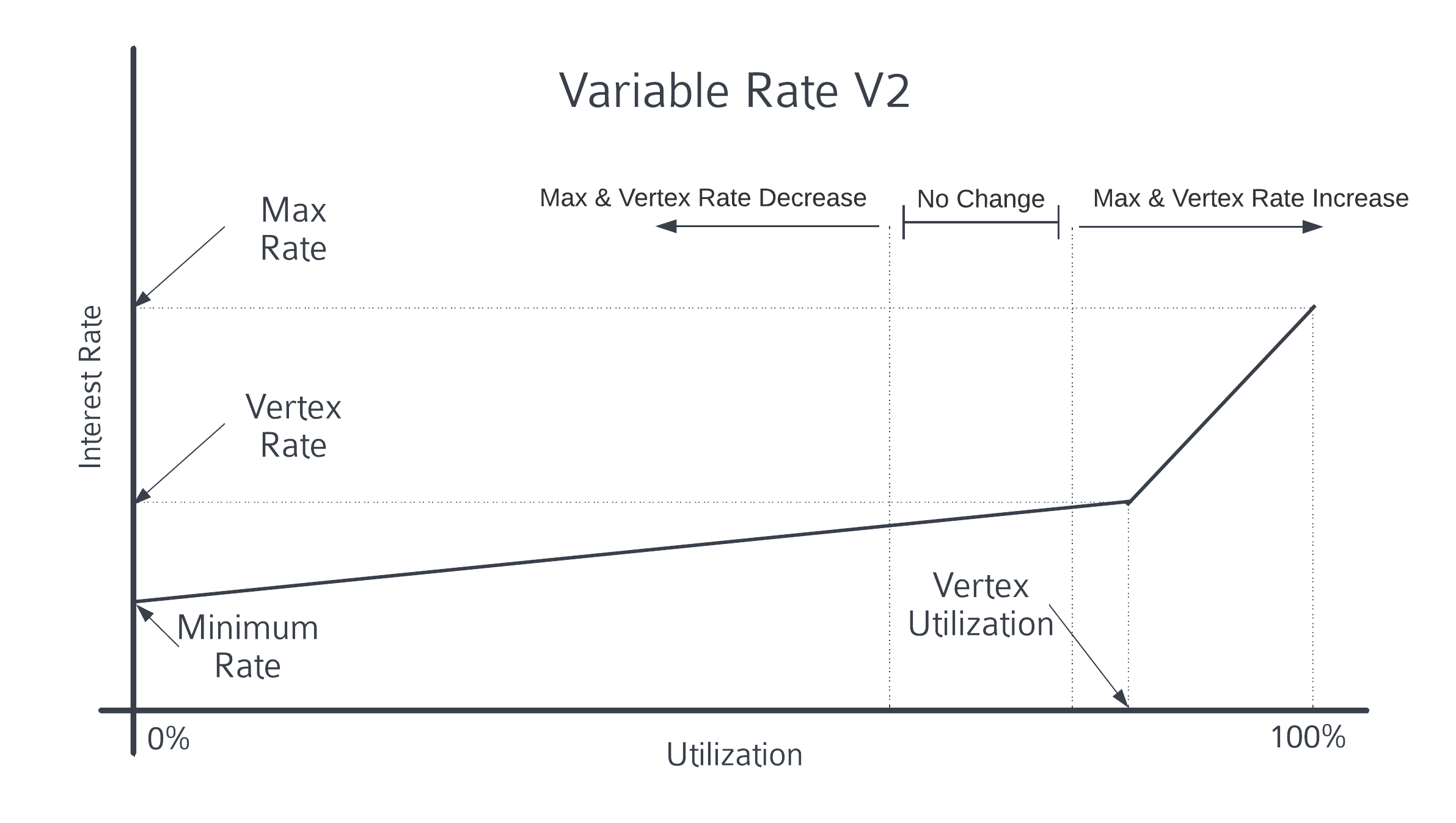
3 Floating Rate V2
Floating Rate V2 combines linear and time-weighted models. It uses a linear function to determine current rate but applies time-weighted formulas to adjust the kink and max rates. Rates respond immediately to utilization changes on the linear curve, while the curve’s slope adapts to long-term market conditions.
Like the time-weighted model, it uses half-life and target utilization range. Low utilization reduces kink and max rates; high utilization increases them.
Rate reductions/increases depend on utilization and half-life. At 0% utilization, kink and max rates halve per half-life; at 100%, they double.
Fraxlend Mechanism – Dynamic Debt Restructuring
In typical lending markets, once LTV exceeds max LTV (usually 75%), liquidators can close positions. But during extreme volatility, liquidators may fail to act before LTV hits 100%, resulting in bad debt—leading to a “race to exit,” where the last to withdraw suffers most.
In Fraxlend, when bad debt occurs, losses are immediately socialized—distributed among all lenders. This preserves market liquidity even after defaults.
Fraxlend AMO
Fraxlend AMO enables minting FRAX into lending markets, allowing anyone to borrow FRAX by paying interest rather than through primary minting.
FRAX minted into money markets does not enter circulation unless borrowers provide overcollateralization, so this AMO does not reduce direct collateral ratio (CR). It helps expand FRAX scale and creates a new distribution channel.
Join TechFlow official community to stay tuned Telegram:https://t.me/TechFlowDaily X (Twitter):https://x.com/TechFlowPost X (Twitter) EN:https://x.com/BlockFlow_News