

Quadratic Arithmetic Programs: A Treatise on Zero-Knowledge Proofs
TechFlow Selected TechFlow Selected
Quadratic Arithmetic Programs: A Treatise on Zero-Knowledge Proofs
Understanding zk-SNARKs is indeed quite challenging, especially because the entire system involves too many moving parts that need to be assembled to work together.
Author: Vitalik Buterin
Published: December 10, 2016
Recently, there has been significant interest in the technology behind zk-SNARKs (zero-knowledge proofs), with growing efforts to demystify what many refer to as "moon math" due to its perceived complexity.
Understanding zk-SNARKs is indeed quite challenging, especially because so many moving parts must be assembled for the entire system to function. However, if we break down this technology piece by piece, it becomes much easier to grasp.
The purpose of this article is not to serve as a complete introduction to zk-SNARKs; it assumes you have the following background knowledge:
1- You are familiar with zk-SNARKs and their general principles;
2- You have sufficient mathematical knowledge to understand basic polynomial concepts. (For example, if P(x) + Q(x) = (P + Q)(x), where P and Q represent polynomials, and you're comfortable with such notation, then you meet the prerequisites for continuing.)

zk-SNARK knowledge pipeline diagram, by Eran Tromer
As shown above, zero-knowledge proofs can be divided into two stages from top to bottom. First, zk-SNARKs cannot be directly applied to any computational problem; instead, you must convert the problem into the correct "form" of operations. This form is known as a "Quadratic Arithmetic Program" (QAP), and converting function code into this form is an important process in itself. Alongside the process of converting function code into a QAP runs another process that allows one to create a corresponding solution (sometimes called a "witness" of the QAP) given an input to the code. This is what this article will cover.
Afterward, there's another rather complex process to generate the actual "zero-knowledge proof" for this QAP, and a separate process to verify someone else's proof when they send it to you—but these details go beyond the scope of this article.
In the example below, we'll choose a very simple problem:
Solve a cubic equation: x**3 + x + 5 == 35 (Hint: The answer is 3).
This problem is simple but illustrative—you can see how all the components work through this case.
Describing the above equation in a programming language:
def qeval(x):
y = x**3
return x + y + 5
The simple programming language used here supports basic arithmetic (+, -, *, /), identity powers (e.g., x^7, but not x*y), and variable assignment. It’s powerful enough that, in theory, any computation can be performed within it (as long as the number of computational steps is bounded—loops are not allowed). Note that modulo (%) and comparison operators (<, >, ≤, ≥) are not supported because there’s no efficient way to perform modulo or direct comparisons over finite cyclic groups (thankfully; if there were a way, elliptic curve cryptography could be broken faster than via “binary search” and “Chinese remainder theorem”).
You could extend the language to support modulo and comparisons using bit decomposition (e.g., 13 = 2**3 + 2**2 + 1 = 8 + 4 + 1) as auxiliary inputs, proving correctness of the decomposition and performing math in binary circuits. Performing equality (==) checks in finite field arithmetic is also feasible—and actually easier—but we won’t discuss either detail now. We could also extend the language to support conditional statements (e.g., converting the statement: if x < 5: y = 7; else: y = 9; into arithmetic form: y = 7 * (x < 5) + 9 * (x >= 5)), though note that both "paths" of the condition must be executed, which could lead to significant overhead if there are many nested conditions.
Now let’s walk through this process step by step. If you want to code any of this yourself, I’ve implemented a version in Python here (for educational purposes only—not ready for generating QAPs for real-world zk-SNARKs!)
Step 1: Flattening
The first step is a "flattening" process, where we decompose the original code (which may contain arbitrarily complex statements and expressions) into the simplest kinds of expressions, which come in two forms:
1- x = y (where y can be a variable or a number)
2- x = y (op) z (where op can be +, -, *, /, and y and z can be variables, numbers, or sub-expressions).
You can think of these expressions as logic gates in a circuit. The flattened version of the expression x**3 + x + 5 looks like this:
sym_1 = x * x
y = sym_1 * x // effectively computes y = x**3
sym_2 = y + x
~out = sym_2 + 5
Each of the above lines can be thought of as a logic gate in a circuit. Compared to the original code, we've introduced two intermediate variables sym_1 and sym_2, plus a redundant output variable ~out. It's clear that the sequence of flattened statements is equivalent to the original code.
Step 2: Convert to R1CS
Now, we convert this into something called an R1CS (Rank-1 Constraint System). An R1CS is a sequence of three vectors (a, b, c), and a solution to an R1CS is a vector s that satisfies the equation:
s . a * s . b - s . c = 0
where . denotes the inner product operation.
For example, the following is a valid R1CS:
a = (5,0,0,0,0,1),
b = (1,0,0,0,0,0),
c = (0,0,1,0,0,0),
s = (1,3,35,9,27,30),
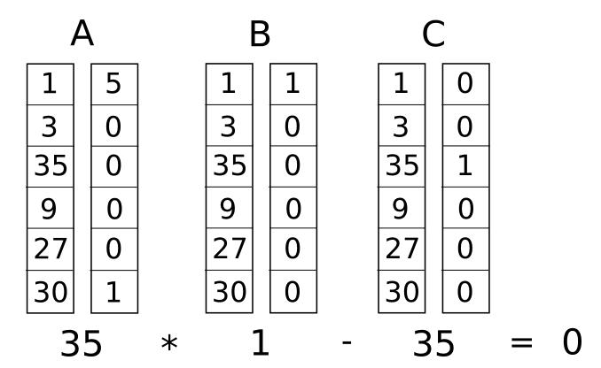
(Translator’s note: 35 = 1*5 + 30*1 for the first equation, and 35 = 35 * 1 for the second)
The above example shows just one constraint. Next, we’ll convert each logic gate (i.e., each flattened declaration) into a constraint (i.e., a triple of vectors (a, b, c)). The method depends on the type of operation (+, -, *, /) and whether the operands are variables or constants. In our example, besides the five flattened variables ('x', '~out', 'sym_1', 'y', 'sym_2'), we need to introduce a dummy variable ~one at the first position to represent the constant 1. For our system, the six components of a vector correspond to (order may vary as long as consistent):
'~one', 'x', '~out', 'sym_1', 'y', 'sym_2'
First gate
sym_1 = x * x → x*x - sym_1 = 0
We get the following vectors:
a = [0, 1, 0, 0, 0, 0]
b = [0, 1, 0, 0, 0, 0]
c = [0, 0, 0, 1, 0, 0]
If the second component of solution vector s is 3 and the fourth is 9, the constraint holds regardless of other values, because: a = 3*1, b = 3*1, c = 9*1 → a*b = c. Similarly, if the second component is 7 and the fourth is 49, it also passes—the first check simply verifies consistency between the first gate’s inputs and outputs.
Second gate
y = sym_1 * x → sym_1 * x - y = 0
Yields the following vectors:
a = [0, 0, 0, 1, 0, 0]
b = [0, 1, 0, 0, 0, 0]
c = [0, 0, 0, 0, 1, 0]
Third gate
sym_2 = y + x → (x + y) * 1 - sym_2 = 0
Yields the following vectors:
a = [0, 1, 0, 0, 1, 0]
b = [1, 0, 0, 0, 0, 0] // corresponds to constant 1, using ~one
c = [0, 0, 0, 0, 0, 1]
Fourth gate
~out = sym_2 + 5 → (sym_2 + 5) * 1 - ~out = 0
Yields the following vectors:
a = [5, 0, 0, 0, 0, 1]
b = [1, 0, 0, 0, 0, 0]
c = [0, 0, 1, 0, 0, 0]
Now suppose x = 3. From the first gate, sym_1 = 9; second gate, y = 27; third gate, sym_2 = 30; fourth gate, ~out = 35. Thus, according to the order: '~one', 'x', '~out', 'sym_1', 'y', 'sym_2', we get:
s = [1, 3, 35, 9, 27, 30]
Different values of x yield different s vectors, but all such s vectors satisfy the constraints (a, b, c).
Now we have four constraints forming an R1CS. The complete R1CS is:
A
[0, 1, 0, 0, 0, 0]
[0, 0, 0, 1, 0, 0]
[0, 1, 0, 0, 1, 0]
[5, 0, 0, 0, 0, 1]
B
[0, 1, 0, 0, 0, 0]
[0, 1, 0, 0, 0, 0]
[1, 0, 0, 0, 0, 0]
[1, 0, 0, 0, 0, 0]
C
[0, 0, 0, 1, 0, 0]
[0, 0, 0, 0, 1, 0]
[0, 0, 0, 0, 0, 1]
[0, 0, 1, 0, 0, 0]
Step 3: From R1CS to QAP
The next step is to convert this R1CS into QAP form, which implements the same logic but uses polynomials instead of inner products. We do this by transforming 4 sets of 3 vectors of length 6 into 6 sets of 3 polynomials of degree 3, where evaluating the polynomials at each x-coordinate represents a constraint. That is, evaluating the polynomials at x=1 gives the first set of vectors, at x=2 gives the second, and so on.
We use Lagrange interpolation for this transformation. Lagrange interpolation solves the problem: given a set of points (i.e., (x,y) coordinate pairs), find a polynomial passing through all of them. We break the problem down: for each x-coordinate, we create a polynomial that takes the desired y-value at that x and zero at all other x-coordinates of interest, then sum all such polynomials to get the final result.
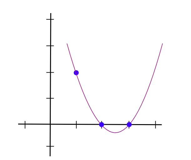
Let’s take an example. Suppose we want a polynomial passing through (1,3), (2,2), and (3,4). First, create a polynomial passing through (1,3), (2,0), (3,0). A polynomial that "peaks" at x=1 and is zero elsewhere is easy—we can use:
y = (x - 2) * (x - 3)
As shown below:
Then, "stretch" vertically using:
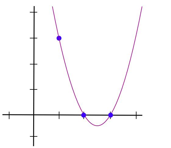
y = (x - 2) * (x - 3) * 3 / ((1 - 2) * (1 - 3))
Simplifying:
y = 1.5 * x**2 - 7.5 * x + 9
Which passes through (1,3), (2,0), (3,0)—see below:
Substituting (2,2) and (3,4) into the formula yields:
y = 1.5 * x**2 - 5.5 * x + 7
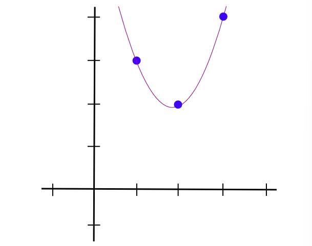
Which is our desired polynomial. The above algorithmrequires O(n³) time, as there are n points and each requires O(n²) time to multiply polynomials. With some thought, this can be reduced to O(n²); with more advanced techniques like fast Fourier transform, it can be further optimized—a crucial consideration when zk-SNARKs often involve thousands of gates.
Here is the Lagrange interpolation formula:
The degree-(n−1) polynomial passing through n points (x₁,y₁), (x₂,y₂), ..., (xₙ,yₙ) is:
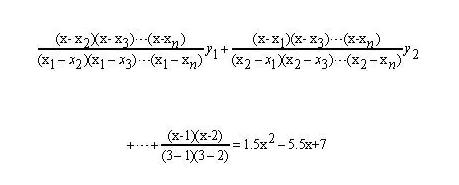
For example, the polynomial through (1,3), (2,2), (3,4) is:
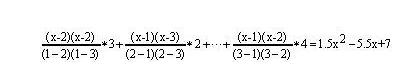
Once you know how to use this formula, we can proceed. Now we convert four triples of length-six vectors into six sets of polynomials, each containing three degree-3 polynomials. We evaluate different constraints at different x-values. Since we have four constraints, we use x = 1,2,3,4 to represent them.
Now we apply Lagrange interpolation to convert the R1CS into QAP form. We first find the polynomial for the first element of each a-vector across the four constraints—that is, the polynomial passing through (1,0), (2,0), (3,0), (4,0). Similarly, we compute polynomials for each i-th element of every vector across the four constraints.
Here are the results:
A polynomials
[-5.0, 9.166, -5.0, 0.833]
[8.0, -11.333, 5.0, -0.666]
[0.0, 0.0, 0.0, 0.0]
[-6.0, 9.5, -4.0, 0.5]
[4.0, -7.0, 3.5, -0.5]
[-1.0, 1.833, -1.0, 0.166]
B polynomials
[3.0, -5.166, 2.5, -0.333]
[-2.0, 5.166, -2.5, 0.333]
[0.0, 0.0, 0.0, 0.0]
[0.0, 0.0, 0.0, 0.0]
[0.0, 0.0, 0.0, 0.0]
[0.0, 0.0, 0.0, 0.0]
C polynomials
[0.0, 0.0, 0.0, 0.0]
[0.0, 0.0, 0.0, 0.0]
[-1.0, 1.833, -1.0, 0.166]
[4.0, -4.333, 1.5, -0.166]
[-6.0, 9.5, -4.0, 0.5]
[4.0, -7.0, 3.5, -0.5]
Coefficients are listed in ascending order; for example, the first polynomial is 0.833*x³ - 5*x² + 9.166*x - 5. Evaluating all 18 polynomials at x=1 recovers the first constraint’s vectors:
(0, 1, 0, 0, 0, 0),
(0, 1, 0, 0, 0, 0),
(0, 0, 0, 1, 0, 0),
...
Similarly, evaluating at x=2,3,4 recovers the rest of the R1CS.
Step 4: Checking the QAP
By converting R1CS to QAP, we can simultaneously check all constraints via polynomial inner products, instead of checking each one individually as in R1CS. As illustrated:
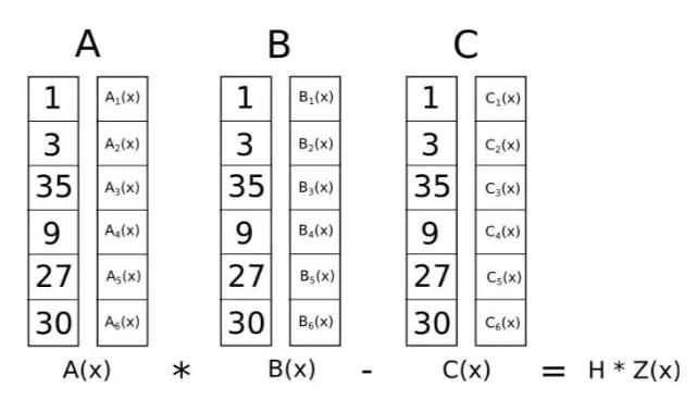
Since the dot product check involves adding and multiplying polynomials, the result is itself a polynomial. If this resulting polynomial evaluates to zero at every x-coordinate corresponding to a logic gate, all checks pass. If it has any nonzero value, the inputs and outputs across logic gates are inconsistent.
Notably, the resulting polynomial doesn't need to be identically zero—in most cases it isn't. It can behave arbitrarily at points not corresponding to any gate, as long as it is zero at all gate points. To verify correctness, we don’t evaluate the polynomial t = A·s * B·s - C·s at each gate point. Instead, we divide t by another polynomial Z and check whether Z divides t evenly—i.e., t / Z has no remainder.
Z is defined as (x - 1)*(x - 2)*(x - 3)*… — the simplest polynomial that equals zero at all gate points. A fundamental fact in algebra states that any polynomial zero at all these points must be a multiple of this minimal polynomial. If a polynomial is a multiple of Z, it evaluates to zero at all those points—this equivalence makes our task much easier.
Now let’s perform the dot product test with the polynomials above.
First, compute intermediate polynomials:
A · s = [43.0, -73.333, 38.5, -5.166]
B · s = [-3.0, 10.333, -5.0, 0.666]
C · s = [-41.0, 71.666, -24.5, 2.833]
(Translator’s note: Calculation:
43.0 = -5*1 + 8*3 + 0*35 -6*9 +4*27 -1*30,
-73.333 = 9.166*1 -11.333*3 +0*35 +9.5*9 -7*27 +1.833*30,
...
-3 = 3*1 -2*3 +0*35 +0*9 +0*27 +0*30
...)
Compute t = A·s * B·s - C·s:
t = [-88.0, 592.666, -1063.777, 805.833, -294.777, 51.5, -3.444]
(Translator’s note: Calculation:
A·s = [43.0, -73.333, 38.5, -5.166] = -5.166*x³ + 38.5*x² -73.333*x + 43,
B·s = [-3.0, 10.333, -5.0, 0.666] = 0.666*x³ -5*x² +10.333*x -3.0,
C·s = [-41.0, 71.666, -24.5, 2.833] = 2.833*x³ -24.5*x² +71.666*x -41.0
Multiplying and subtracting gives t, with coefficients ordered from lowest to highest power: [-88.0, 592.666, -1063.777, 805.833, -294.777, 51.5, -3.444])
Click here to view calculation
The minimal polynomial is:
Z = (x - 1) * (x - 2) * (x - 3) * (x - 4)
That is:
Z = [24, -50, 35, -10, 1]
Click here to view calculation
Now compute polynomial division:
h = t / Z = [-3.666, 17.055, -3.444]
h must divide evenly with no remainder.
Click here to verify backwards
We now have a solution to the QAP. If we try to forge a variable in the R1CS that leads to the QAP solution—say, setting the last entry of s to 31 instead of 30—we get a t polynomial that fails the check (in this case, t(3) = 1 ≠ 0) and is not divisible by Z; dividing t/Z would leave a remainder of [-5.0, 8.833, -4.5, 0.666].
Note that the above is just a very simple example. In real-world applications, addition, subtraction, multiplication, and division usually involve non-standard numbers, so all the algebraic rules we know and love still apply—but all results are elements of some finite field, typically integers modulo a prime n, ranging from 0 to n−1. For instance, if n = 13, then 1/2 = 7 (since 7*2 ≡ 1 mod 13), 3*5 = 2, etc. Using finite field arithmetic eliminates concerns about rounding errors and enables compatibility with elliptic curves, which is ultimately essential for making zk-SNARK protocols truly secure.
Join TechFlow official community to stay tuned
Telegram:https://t.me/TechFlowDaily
X (Twitter):https://x.com/TechFlowPost
X (Twitter) EN:https://x.com/BlockFlow_News